Project Setup
Overview
In order to make creating new projects easy, Percept incorporates a project setup wizard, a software component which guides you through the different steps needed in order to set up your own Project.
These steps are:
-
Step 2 - Registration of multiple LiDAR devices (optional) if you are using Percept for a multi-LiDAR setup.
-
Step 4 - Zone Management in order to setup areas of interest for e.g. object detection.
-
Step 5 - Configure Advanced Settings and select algorithm parameters for fine tuning Percept’s behaviour.
-
Step 6 - Define Output Options for data generated by Percept.
-
Step 7 - Manage existing Projects for your generated project.
Step 1 - Create a Project
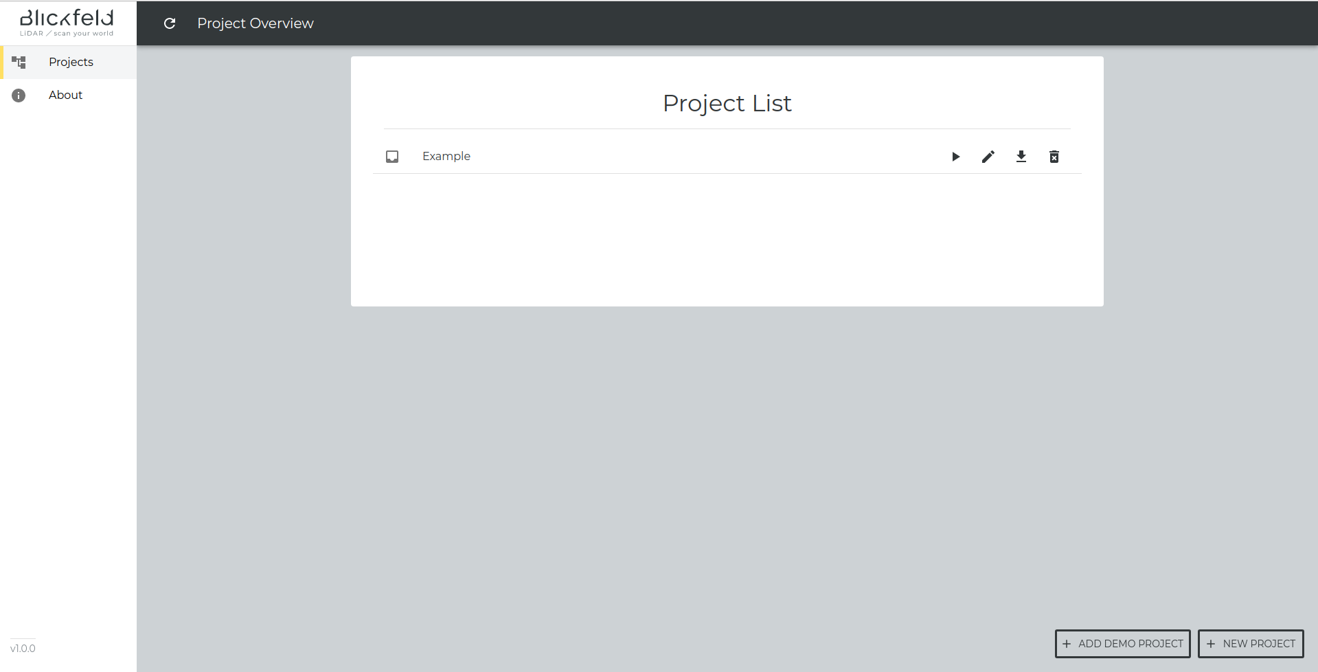
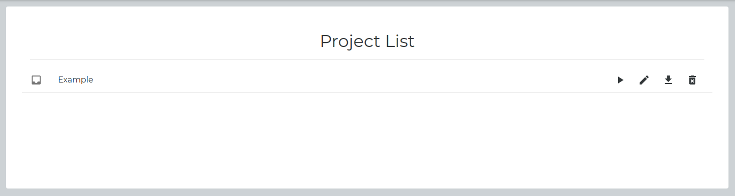
The first time Percept is accessed over the browser (see also Access Percept Web Interface), it will show the project view with an empty project list. The project overview shows the list of your created projects.
In order to create a new project, you will have to click on "New Project" on the lower right corner of the browser window. This will open the project setup wizard, as detailed in Create a New Project. As an alternative, it is possible to create a demo project by clicking on "Add Demo Project". These projects are completely pre configured and ready to be used, as explained in Create a Demo Project.
Create a New Project
Enter General Project Information
After clicking on the "New Project" button, the project wizard is started and it will bring you to the basic project information configuration screen. Here you need to define:
-
A name for the project (cannot be changed later on).
-
The LiDAR devices to use in your project.
-
A name, e.g. cube_front_entrance in order to easily distinguish between different devices and have an indication for the location of your LiDAR.
-
The IP-address/Hostname of the LiDAR connected to your network.
-
-
To get familiar with Percept, we provide example recordings. Therefore, choose as data source Example Point Cloud Recording and select an example instead of using a Connected Lidar. The example recordings will be played in an infinite loop.
| The IP-address/Hostname of the LiDAR can be found within the Web GUI of the LiDAR device itself. Please refer to the user manual of the device in order to understand how to access the device’s Web GUI. |
After choosing a project name and adding the LiDAR devices to your project, click on "Create Project" to continue with the wizard. If you click on the "X" in the top left corner, you will abort the project setup and get redirected to the project overview page.
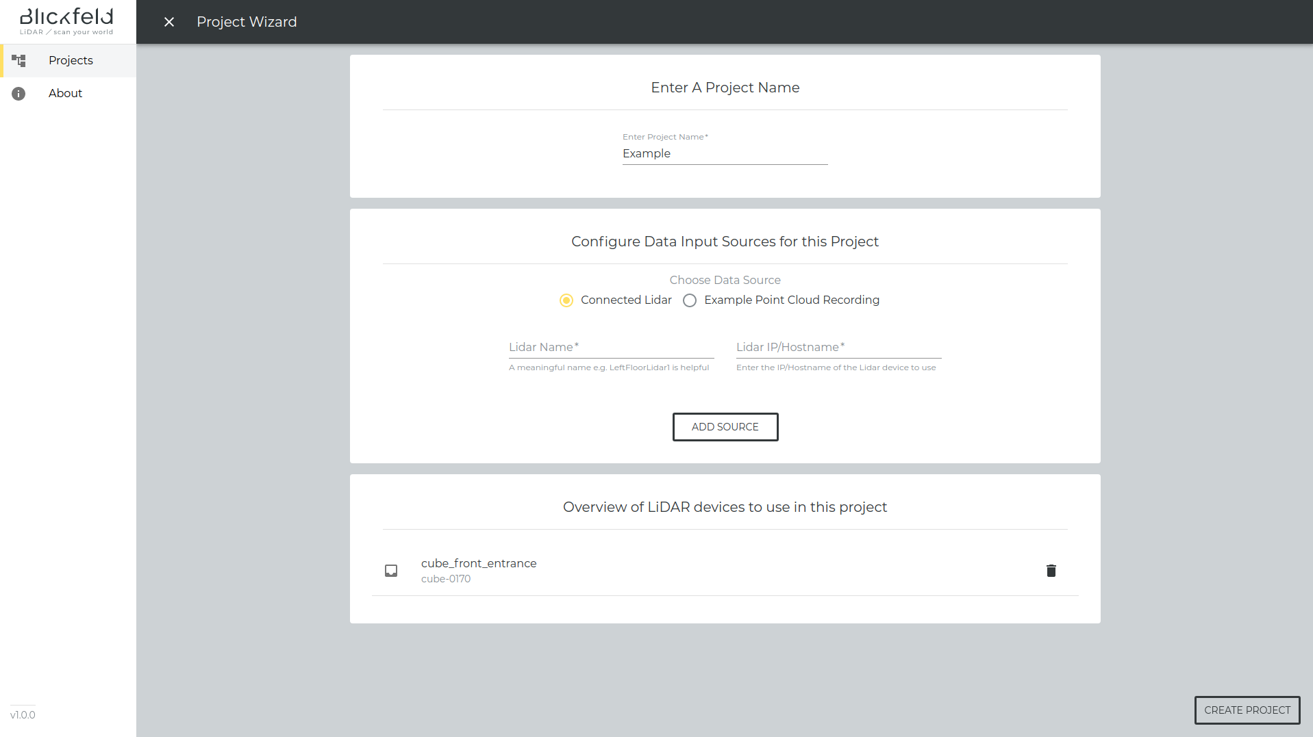
| Make sure that the LiDAR devices you want to use are shown in the Input Sources To Use In This Project, you can remove devices from the list as well. |
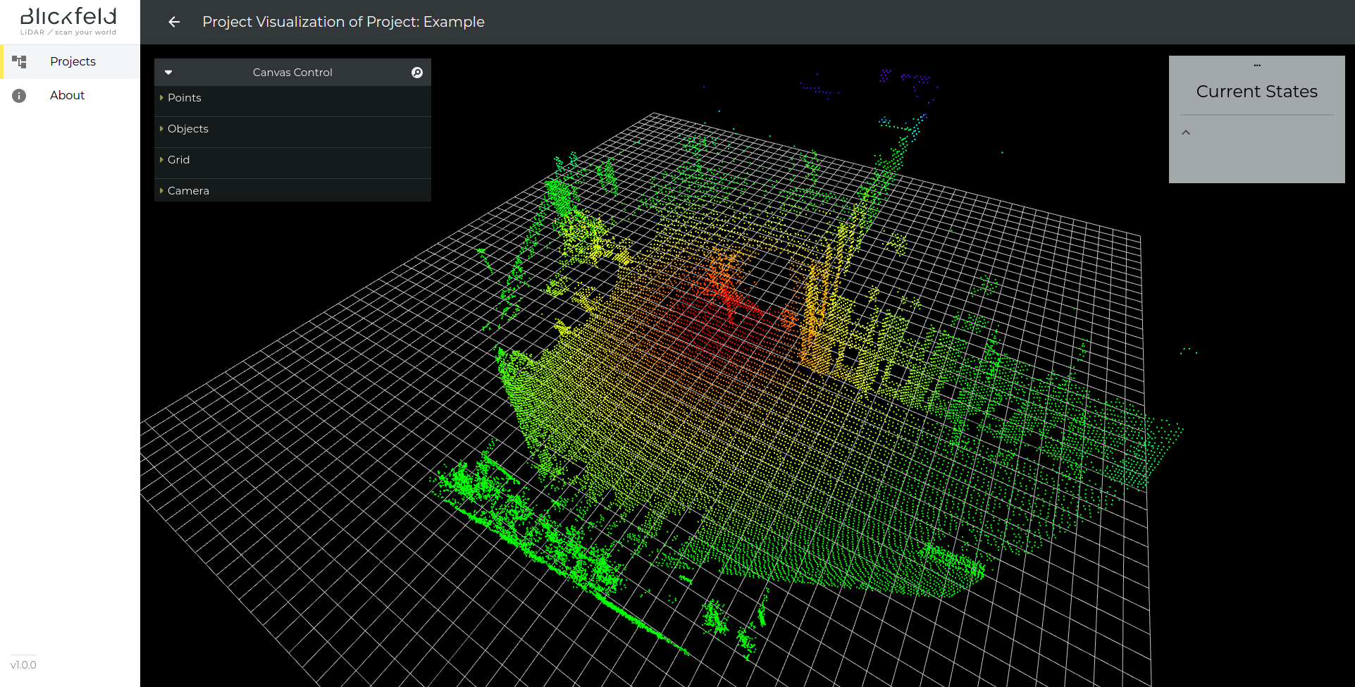
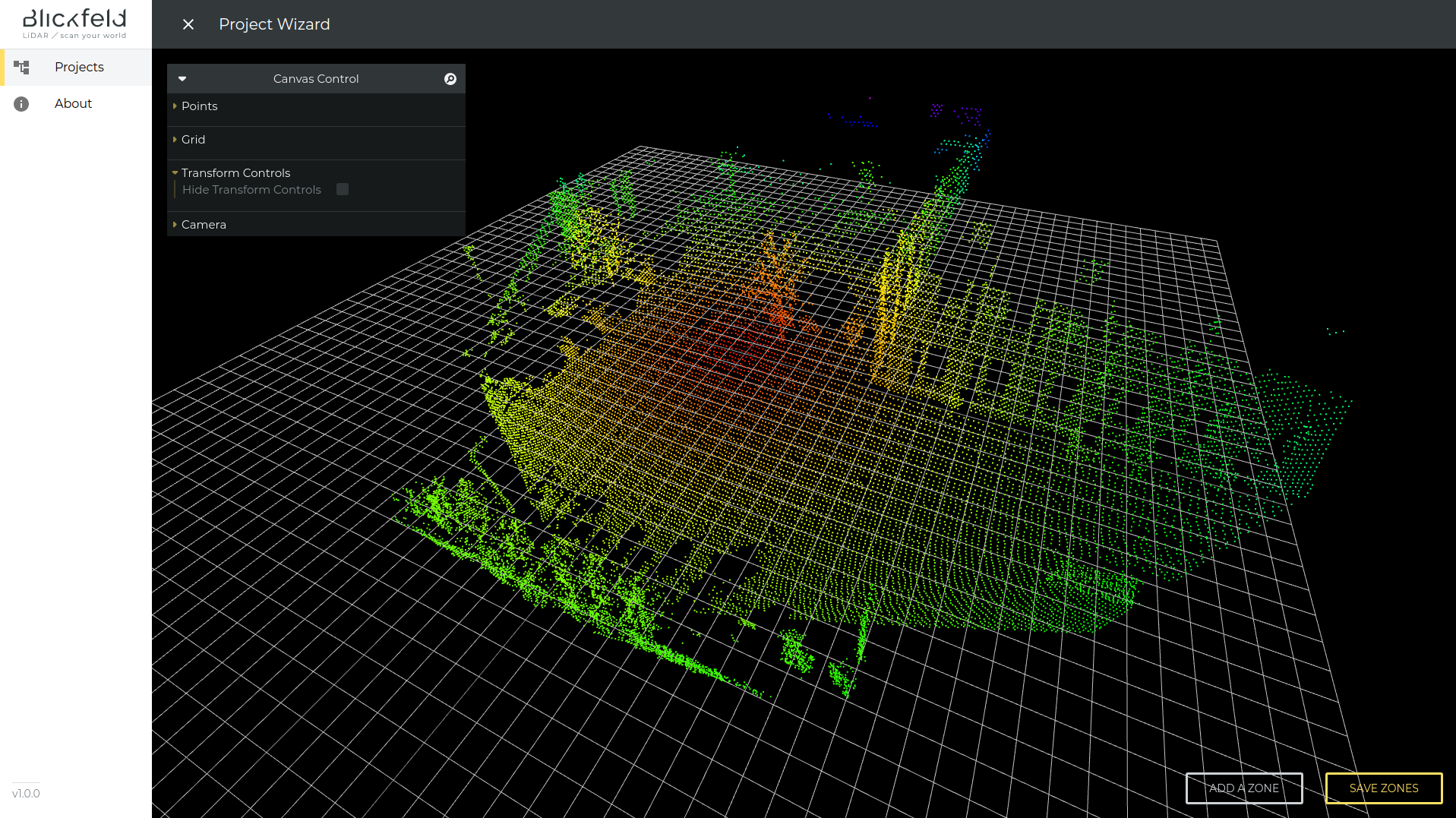
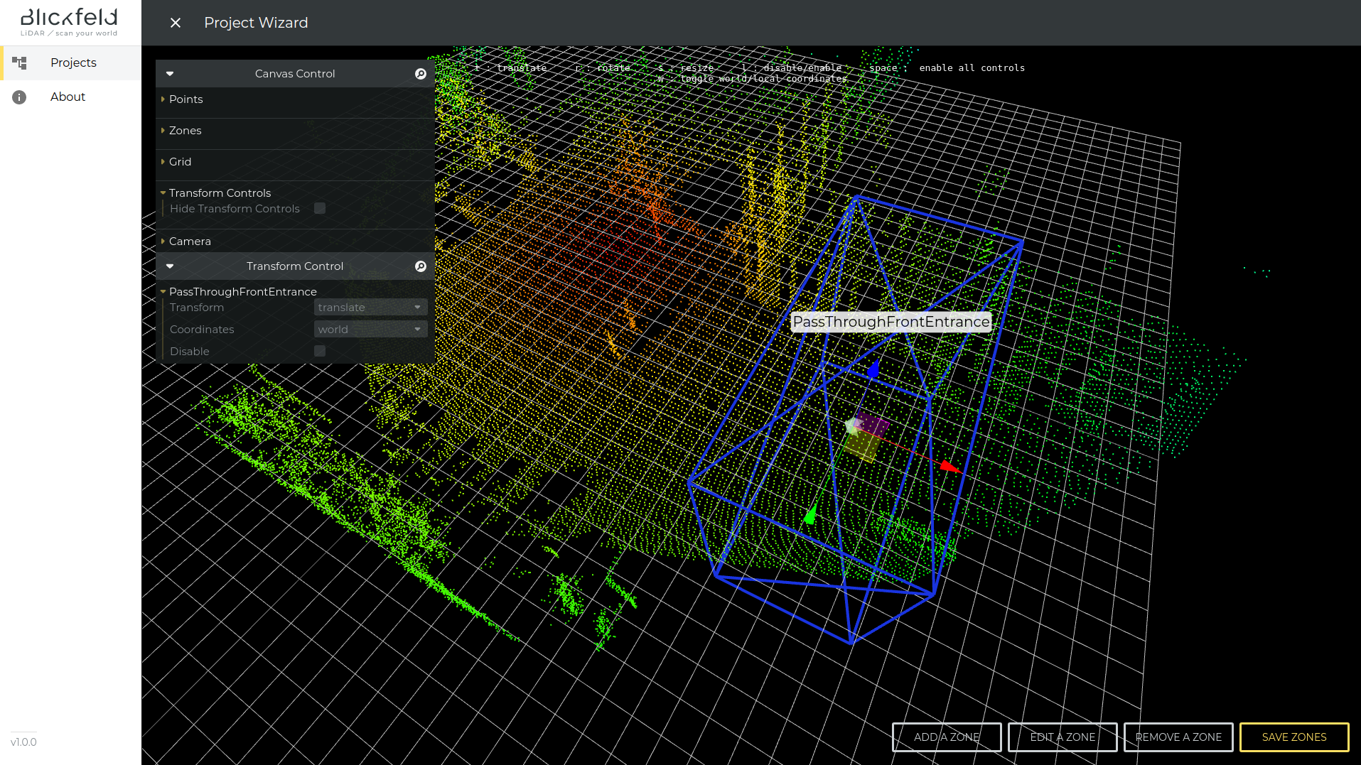
3D Viewer Overview
The 3D Viewer is a shared visualization tool between the project wizard and the project visualization.
It will show you the point cloud(s) generated by the device(s) used.
|
You can rotate and translate the camera in the 3D scene and also zoom in and out of the scene.
|
You can change the camera view on the 3D scene with the following mouse interaction:
|
There is a control window, which lets you adjust the visualization to your needs.
-
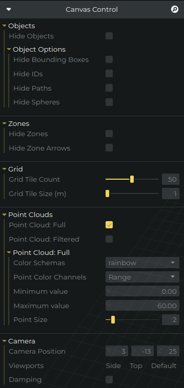
Objects
-
Hide Objects will disable the visualization of the detected objects
-
Object Options
-
Hide Bounding Boxes will disable the visualization of the object bounding boxes
-
Hide IDs will disable the visualization of the object ID
-
Hide Paths will disable the visualization of the object path
-
Hide Spheres will disable the visualization of the sphere marking a detected object
-
-
-
Zones
-
Hide Zones will disable the visualization of the zones
-
Hide Zone Arrows will disable the visualization of the direction indication with zone arrows
-
-
Grid
-
Grid Tile Count selects the amount of tiles for the grid
-
Grid Tile Size (m) selects the size of each grid cell in meter
-
-
Point Clouds
-
Point Cloud: Full will disable the visualization of the point clouds
-
Point Cloud: Filtered will enable the visualization of the foreground points generated by the background subtraction
-
Point Cloud: Full
-
Color Schemas selects the coloring method for the point cloud
-
Point Color Channels The channel to use for coloring, e.g. range
-
Minimum value The minimum value of the point color channel to start with the coloring, everything smaller will get mapped to the same color
-
Maximum value The maximum value of the point color channel to start with the coloring, everything above will get mapped to the same color
-
Point Size will adjust the point size of the point clouds displayed
-
-
-
Camera
-
Camera Position sets the camera position
-
Viewports selects a fixed camera viewpoint (Side, Top, Default)
-
Damping when active, if you move the camera around it will continue the movement and slowly stops
-
| Not all of the options mentioned above will always be available. |
Create a Demo Project
By clicking on "Add Demo Project" in the lower right corner of the project list window, it is possible to create a project that is already pre configured. Demo projects are available to showcase some potential use cases of Percept for various applications and to provide an orientation of how a complete project can look like without the need to go through the setup wizard first.
After clicking on the button, a pop-up is shown. Here, the only needed steps are:
-
Select a name for the project, e.g. example-project-security.
-
Choose one of the available projects based on the application of interest. Currently, these applications are available:
-
Security: a security zone is placed at a crossroads to check if people walk through it.
-
People Counting: two pass-through zones are used to count the number of people walking down two different streets. People are counted based on the direction they walk through the zone.
-
More information about these zones can be found in Step 4 - Zone Management.
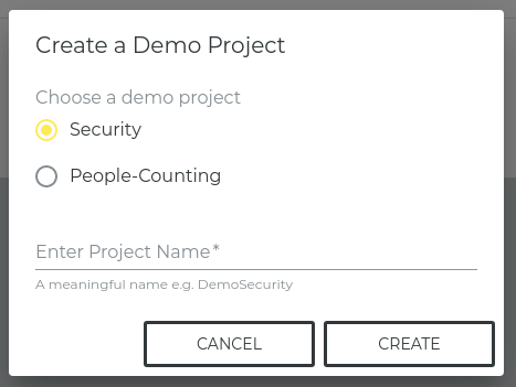
From the pop-up, click "Cancel" to cancel the project creation or "Create" to create the selected demo project. In the second case, the new project can now be seen in the project list and started directly, as explained in Step 7 - Manage existing Projects.
| A "_demo" suffix is added to the chosen project name to distinguish the demo projects from other projects created using the setup wizard. |
Step 2 - Registration of multiple LiDAR devices (optional)
If your setup consists of multiple LiDAR devices, the project wizard will bring up the registration step after the initial project information screen. Registration entails that we will combine multiple point clouds from different devices to a single unified point cloud, by finding the position and orientation of the devices with respect to each other. This is necessary to combine multiple sensor measurements, allowing for utilizing their data just as if it were generated by a single sensor with a larger field of view or a higher point cloud density.
| The registration step is only required if you use more than one LiDAR device in your project. |
For the registration of multiple LiDAR devices, you can choose between a marker based and a semi-automatic approach, which will be explained below.
| In both methods the point clouds need to have an overlap in order to be able to register them. |
Marker Based Registration
For marker based registration a spherical object is used as a marker and access to the area in field of view of the lidars is needed. During the registration process the marker needs to be placed in the overlapping area between the corresponding devices. At least three detections of the marker on different positions in the overlapping area are required to reliably register the point clouds. This method works best in a static environment, where only the marker and the person moving the marker to different positions are present.
|
Requirements for Marker Based Registration
|
The marker-based registration shows you two point clouds in parallel, you can select which point clouds you want to display using the drop down menu. Select two point clouds which have an overlap and then start placing the marker in the overlapping area.
Auto Align on Grid
Reset the transformation to automatically align the point cloud on the virtual grid, i.e. move the point cloud on top of the grid and rotate it so the detected ground would be aligned on the grid. It is recommended to use this feature at the start of process to automatically align the point clouds.
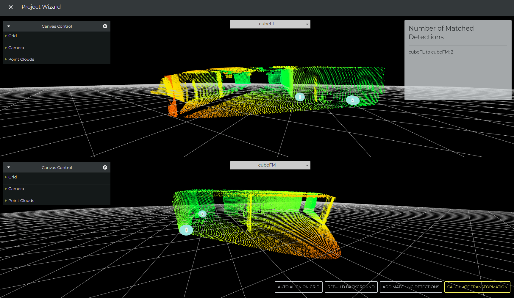
Percept will try to find the marker in the scene. When there is a marker detected, Percept will show you a dark blue sphere at the place where it is detected.
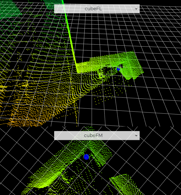
If the sphere shows up in both point clouds, press ADD MATCHING DETECTIONS and it will be saved as a valid match. The sphere in the visualization will turn light blue and gets a number, indicating the matched marker.
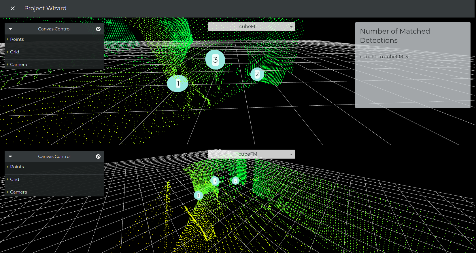
After the match is saved, physically move the marker to another location in the overlapping area and repeat this step until you have at least three matched detections.
If you have enough (best 3 or more) matched detections between all overlapping areas, click on CALCULATE TRANSFORMATION, Percept will then calculate the transformation between all correspondences and display the result in the next step.
| Check the result if it is correct, before you continue with the wizard. If the result is not correct, please go back and try it again. |
-
Make sure that the scene is empty
-
Start the marker based registration and wait around ten seconds until you move into the scene with the marker
-
Place the marker into the scene and make sure it is clearly visible in the corresponding point clouds
-
Make sure that the marker does not move
-
If there is a dark blue sphere in both point clouds, at the place where the marker is, click on ADD MATCHING DETECTION to save this match. The Number of Matched Detections between these two devices will increase by one.
-
Repeat steps (3) to (5) until you have at least three markers per overlapping area
-
Click on "Calculate Transformation"
-
Check the result in the next step, if it is not correct, go back and try it again
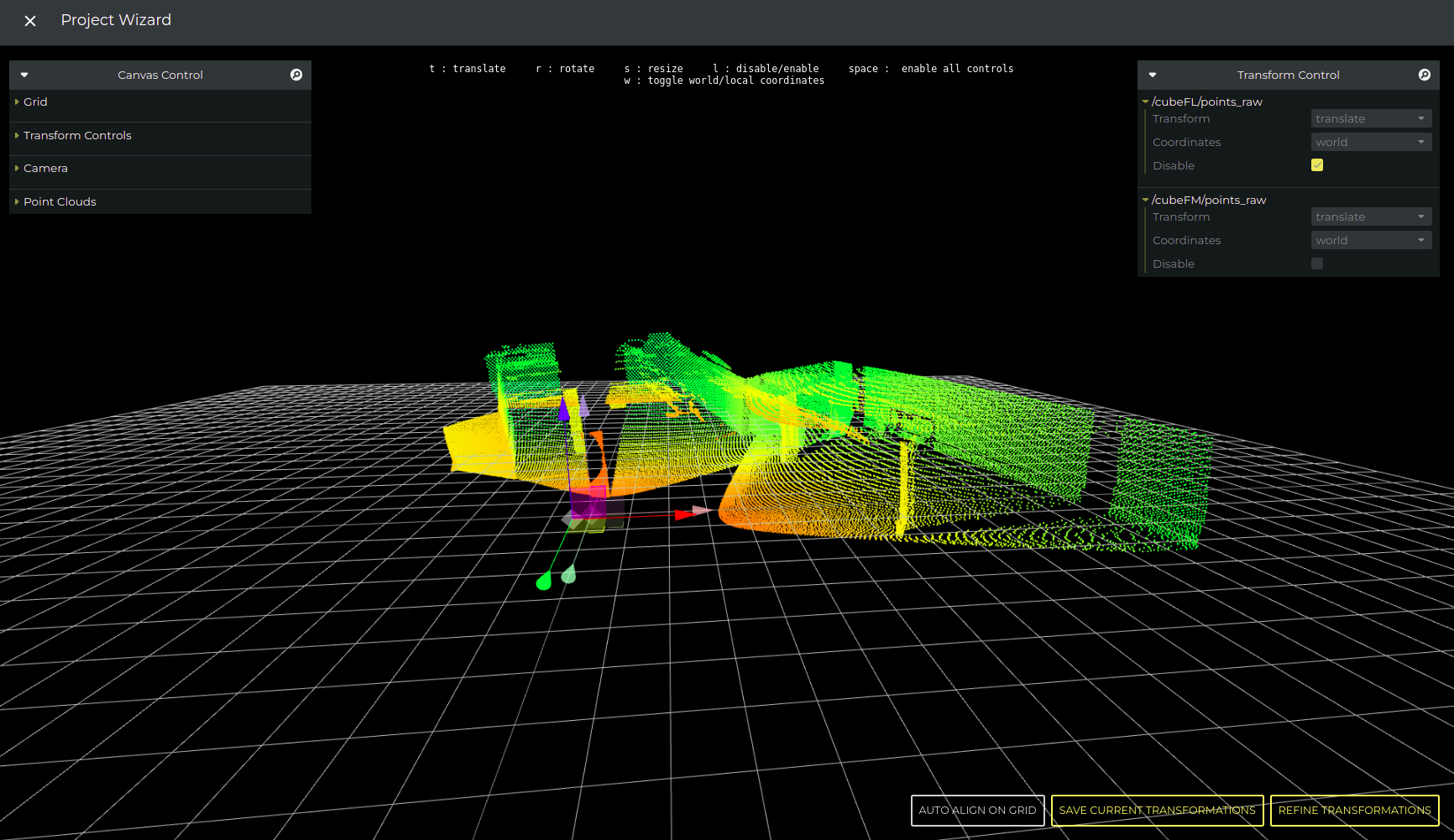
Semi-Automatic Registration
The semi-automatic registration is especially useful in crowded environments, or if you can’t use the marker based methods and in scenarios with not much overlap. If you are used to viewing 3D point clouds it might even be faster than the marker based method.
The semi-automatic method allows the user to transform every point cloud, with the goal of them matching roughly together. Then in the next step, Percept will refine the transformation so that it is accurately registered. In case it is needed, there is also the possibility of skipping the refinement and directly moving on to the next step. In this case, the point clouds will be kept in the manually set positions and no refinement will be applied.
Auto Align on Grid
Reset the transformation to automatically align the point cloud on the virtual grid, i.e. move the point cloud on top of the grid and rotate it so the detected ground would be aligned on the grid. It is recommended to use this feature at the start of process to automatically align the point clouds. Afterwards the alignment can be adjusted if the auto alignment result is not satisfying.
| Refining the transformations is the preferred way to register point clouds. Skipping the refinement is to be avoided, unless the refinement step is not able to improve the registration or in cases where the registration is actually not needed (for example, if multiple LiDAR devices are used but they do not have overlap with each other). |
|
Requirements for Semi-Automatic Registration
|
|
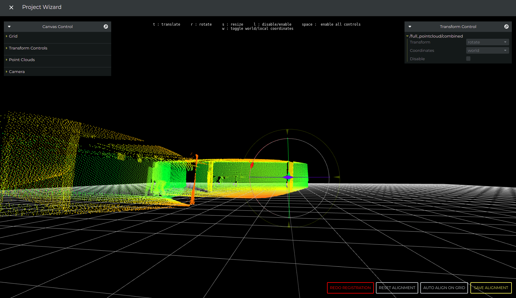
There are two ways to manipulate (transform) the point cloud, 1) using transform control window, 2) using keyboard shortcuts.
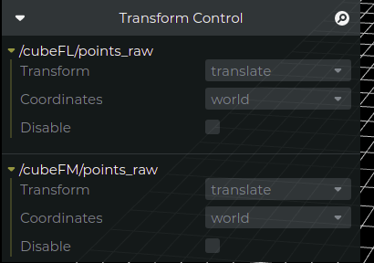
Figure 10. Transform Control Window
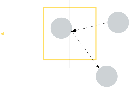
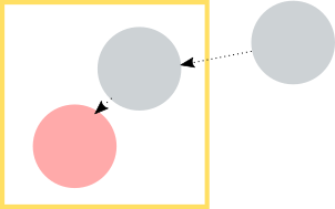
Some useful keyboard shortcuts to transform a point cloud (make sure that you selected the controls for this point cloud):
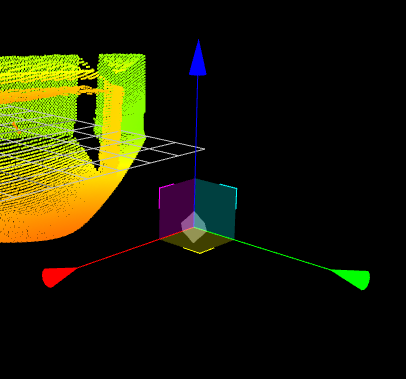
Figure 11. Controls to translate the point cloud
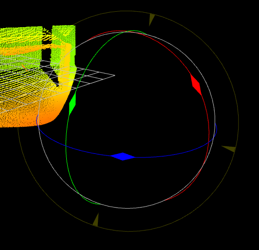
Figure 12. Controls to rotate the point cloud
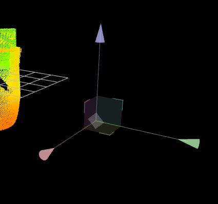
Figure 13. Controls locked
|
|
One tip on how to speed up your workflow
|
-
Select the first point cloud coordinate system by clicking on it
-
Unlock the controls for it
-
Rotate and translate the point cloud, so that the overlapping area fits to the point cloud of the other LiDAR
-
Press "Refine Transformations" (preferred option). As an alternative, press "Save Current Transformations" to avoid applying refinement
-
Check the result in the next step, if it is not correct, go back and try it again
| Have a look at the refinement result before continuing with the project creation. If you are not satisfied with the result you have the chance to go back and try it again. |
Step 3 - Alignment of the Point Cloud on the Virtual Grid
The goal of the alignment step is to align the ground area of the point cloud on the virtual grid. Aligning the ground on the virtual grid will help in zone management step, and it will make it easier to understand the 3D scene. Virtual grid will help in zone management step, will make it easier to understand the 3D scene and is required for good tracking, counting and volume measurement performance.
Redo Registration
Registration step can be done again in case its result is not satisfying. For the new Registration attempt, you can choose whether you want to use the previous transformation or restart from scratch. The registration button will be enabled only for multi sensor setup.
| Using previous transformation is only possible for semi automatic registration |
Reset Alignment
Discard all the changes and reset the point cloud to its initial position.
Auto Align on Grid
Reset the transformation to automatically align the point cloud on the virtual grid, i.e. move the point cloud on top of the grid and rotate it so the detected ground would be aligned on the grid. It is recommended to use this feature at the start of process to automatically align the point clouds. Afterwards the alignment can be adjusted if the auto alignment result is not satisfying.
Save Alignment
If alignment is satisfying, click on "Set Alignment", which will take you to the next step.
| For tracking and object counting/monitoring as well as for volume measurement projects it is required to align the ground to the grid! |
|
You can use the "Align on Grid" function, to align the point cloud on the grid (if the result is not as expected, manually align the point cloud) |
|
There are two ways to manipulate (transform) the point cloud, 1) using transform control window, 2) using keyboard shortcuts.
Figure 15. Transform Control Window
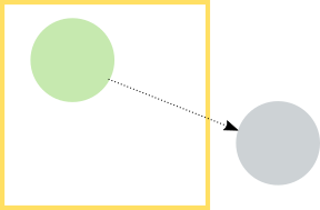
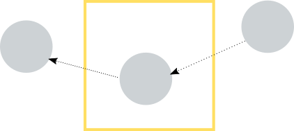
Some useful keyboard shortcuts to transform a point cloud (make sure that you selected the controls for this point cloud):
Figure 16. Controls to translate the point cloud
Figure 17. Controls to rotate the point cloud
Figure 18. Controls locked
|
Step 4 - Zone Management
Percept has different types of detection zones. Detection zones are used to apply certain algorithms to an area of interest in the point cloud, that could be a zone to count if something (e.g. an object) is inside the zone or not. The following section will introduce you to all available types and lay out corresponding example use case.
|
A good mounting position and the right amount of LiDAR devices is important to make the results reliable. For example, if you expect objects to occlude other objects, or there are some obstacles in the field of view, consider changing the mounting position or adding one or more LiDARs from different angles. Since occlusion can have a negative effect on the system performance. |
Pass Through Counter Zone
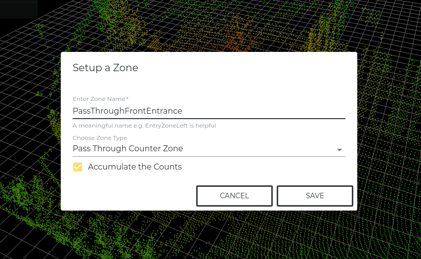
The Pass Through Counter Zone counts the number of objects that moves through the zone in a specific direction. In order for a counting event to trigger, the object needs to start outside the zone, move through the zone and fully exit the zone again. The Pass Through Counter Zone can either accumulate all counted objects or show only the currently counted objects. This can be configured by activating or deactivating the 'Accumulate the Counter Zone' option in the Pass Through Counter Zone definition, as can be seen in Example of the user interface to create a Pass Through Counter zone.
The Zone has a direction to specify what movement will be counted as entry and what movement will be counted as exit (see screenshot below). A movement in the direction of the arrow will be an counted as entry, while a movement in the opposite direction will be counted as an exit.
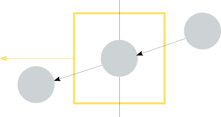
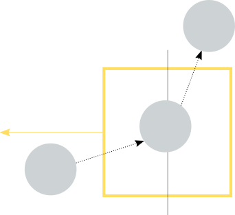
| Objects moving into the zone and disappearing (have a look at the Appearance/Disappearance Counter Zone for this use case) or leaving the zone through the side it entered (seen from the middle of the zone) will not get counted. |
| Please make sure that the LiDAR covers enough area around the zone. Since we need at least one detection before the object enters the zone and one detection after the object leaves the zone for the system to trigger an increase in the inbound or outbound direction |
| Please adjust the width of the zone to allow at least one detection inside of the box (this will depend on the scan pattern and therefore on the framerate and on the object speed), to reliably detect inbound/outbound movements. |
Appearance/Disappearance Counter Zone
The Appearance/Disappearance Counter Zone will count if an object moves into a zone and then disappears (outbound) or if an object appears in a zone and then leaves the zone (inbound). Use cases are e.g. a person entering an elevator or an escalator. Another use case would be the entrance into an area which is not covered by a LiDAR, e.g. a store where you want to count how many people are entering or exiting, but you do not have enough coverage to use a Pass Through Counter Zone. The Appearance/Disappearance Counter Zone can either accumulate all counted objects or show only the currently counted objects. This can be configured by activating or deactivating the 'Accumulate the Counter Zone' option in the Appearance/Disappearance Counter Zone definition. An example of this for the Pass Through Counter Zone is shown in figure Example of the user interface to create a Pass Through Counter zone and for the Appearance/Disappearance Counter Zone there is an equivalent option during the zone creation.
Objects appearing inside the zone and disappearing inside the zone, without leaving the zone will not get counted. Objects entering the zone and leaving the zone will also not get counted.
| Please make sure that the LiDAR covers enough area around the zone. Since there needs to be at least one detection outside of the zone and one detection inside the zone. |
| Please make the zone large enough to allow at least one detection inside the zone. |
Current Objects Counter Zone
The Current Objects Counter Zone counts the amount of detected objects inside a zone for every frame.
| An object is counted if the center of the object is inside the zone. |
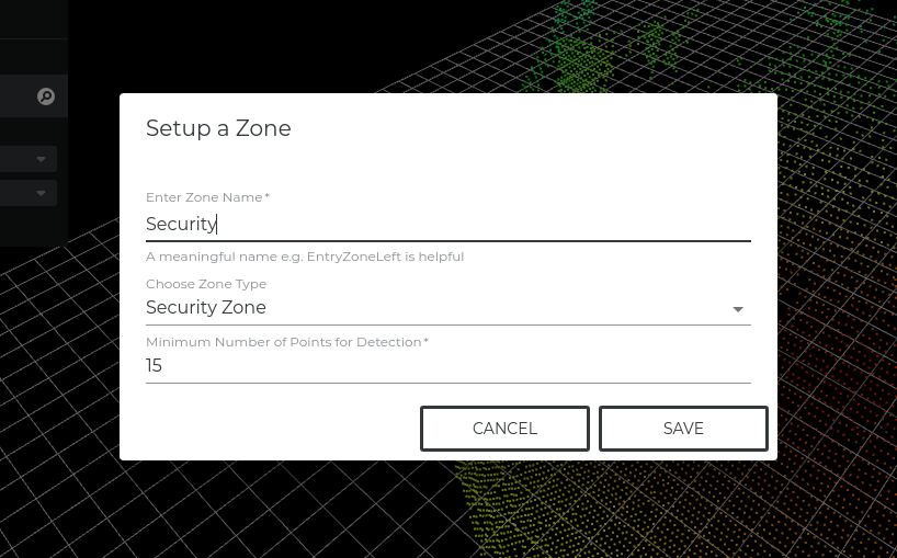
Security Zone
The Security Zone works with points rather than with objects. While an object can consist of e.g. 50 or 100 points, the security zone decides based on the number of points if an intrusion is happening or not. The threshold level defining the minimum number of points before an alarm is raised can be defined by the user.
| The amount of points reflected from an object in the zone will depend on the scan-pattern used by the LiDAR device and therefore needs to be adjusted to prevent false or missed alerts. |
| The amount of points reflected from an object is distance dependent. Think about splitting the zone in multiple ones with different threshold values or adding LiDARs to the scene for a better coverage. |
| It does not matter where the points in the zone are, if the threshold level is exceeded an alarm is raised. |
Occupancy Zone
The Occupancy zone works similar to the Security Zone, with the difference that the output message will be different. This zone is for e.g. parking spot monitoring where you want to get a message that a specific spot is occupied rather than an alarm message.
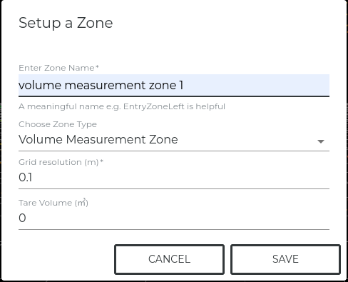
Volume Measurement Zone
The Volume Measurement Zone provides a method to measure the volume inside the zone. It is important that the point cloud is aligned on the grid for the volume measurement zone to work reliably. You can specify the grid resolution used to calculate the volume. The grid resolution will influence how accurate the result is, a smaller grid resolution will therefore be more accurate but it will have higher processing cost. If you have a very large Volume Measurement Zone to improve the performance you could use a higher resolution, otherwise the default resolution should perform well for most use cases. Note that a value smaller then the point to point distance generated in the point cloud will not increase the accuracy.
It is also possible to manually define the tare volume for the zone, this value will be subtracted from the measured total (gross) volume. With this it is possible to remove objects standing around or walls which are not intended to get measured. Also it is possible to measure negative volumes.
| The grid resolution per tile is defined in meter and the volume in cubic meter. |
The option to manually set the tare volume is not only available during the zone setup/edit, but also an automatic option is available during the runtime of the project. If your project contains volume zones, a button will appear on the bottom-right corner of the project visualization page. By clicking on it, a pop up will appear displaying the list of volume zones in the project.
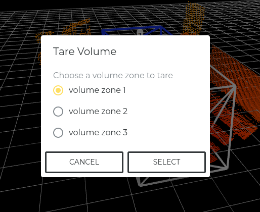
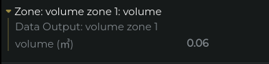
By selecting one of the volume zones, the current total (gross) volume will be displayed.
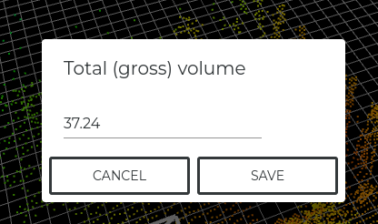
If you click on save, the total (gross) volume will be set as the tare volume for this zone. This will be subtracted from the total (gross) volume and will be displayed in the Zone Output on the top-right corner. This process is similar to manually setting the tare volume of a zone during the setup/edit of the zone but the value can be calculated automatically.
Zone Management Interface
In the project setup and in the project edit mode you can create, delete or change the zones.
If you don’t have a zone created you can either create one or if you don’t want to have a zone at all you can go to the next wizard step with the Save Zones button.
By adding a zone, Percept will open a dialog where you can select the different zone types. Select the zone type and enter a name for your zone. Press "Save" to create the zone.
Now since we created a Pass Through Counter zone make sure that its arrow shows into the direction you want to count as entry, have a look into the Pass Through Counter Zone description for details.
There are now two additional buttons to delete or edit the created zones.
In the transform control panel you will find a copy button for each zone, with which you can create a copy of a zone including the zone type, size and orientation. The copy of the zone will be positioned next to the original zone. A name will be suggested for the new zone but it can be modified to different name if needed.
Add all the zones you need to your project.
| You can mix different zone types in your project. E.g. create one Pass Through Counter zone and one Appearance/Disappearance Counter. |
The Security Zone and Occupancy Zone will have an additional field where you can set the minimum points threshold.
Click on Save Zones to continue with the next wizard step or finish your project edit.
|
Some useful keyboard shortcuts to transform a zone:
|
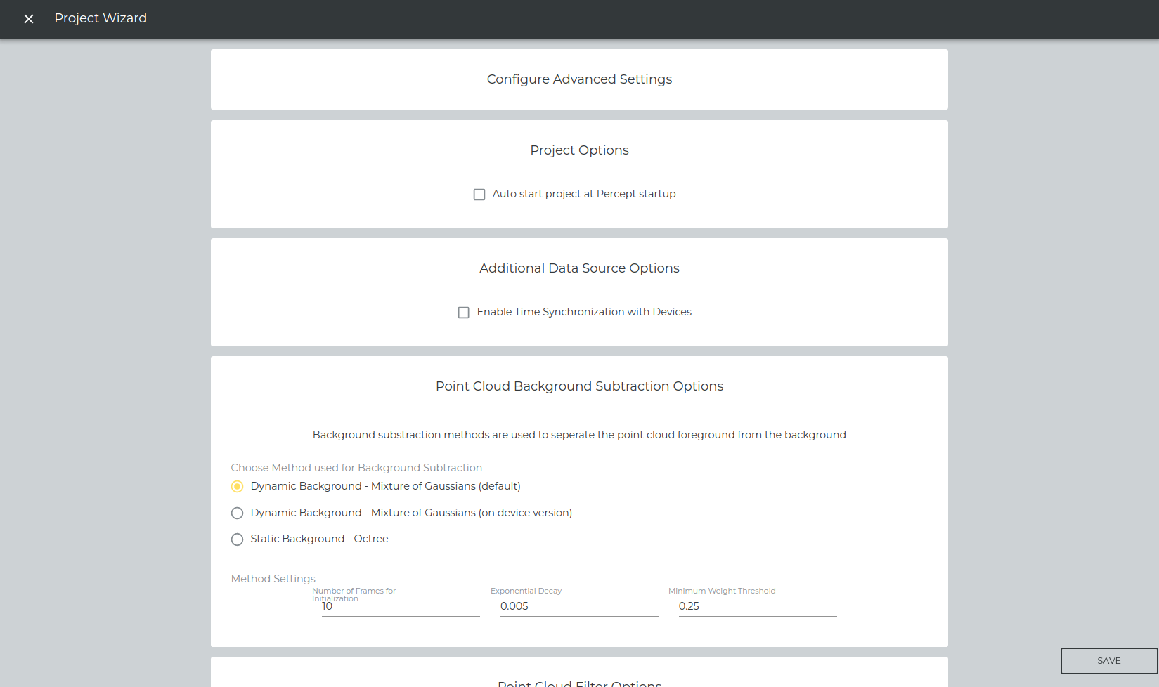
Step 5 - Configure Advanced Settings
In the Advanced Settings you can change the algorithm parameters used by Percept. The default parameters are good for object tracking use cases with slow objects, like people.
If that does not meet your use case you can change the parameters here to improve your result.
The options will be discussed in this section in detail.
Project Options
Here you can select if you want to enable auto starting the project at the start of the Percept. If it is enabled, the project will be automatically initiated on the startup of Percept.
Data Source Options
Here you can select if you want to enable time synchronization of the devices or not. If it is enabled, Percept will synchronize the device/s with an ntp server. This ntp server has to be set in the WebGUI of each LiDAR device.

|
When to use time synchronization:
|
|
If time synchronization fails when starting a project, check in the device WebGUI if these conditions are met:
|
Algorithm Parameter Sets
Parameters, e.g. for Clustering or Tracking, can be optimized to suit your application. By default, the parameters are set to perform good on object tracking use cases with slow objects, like walking people.
With Select Parameter Set you can load parameters for different type of applications. These suggestions are a good starting point for your application and can be further optimized, see the following sections which describe the advanced options in more detail.

Currently we have the following parameter sets:
-
Crowd Analytics (for slow objects, e.g. people, currently the default values)
-
Traffic Monitoring (for faster objects, e.g. cars, bikes)
| With Load Parameters the parameters will not get applied until you click on save in the project wizard. |
Background Subtraction Options
Background subtraction is used to separate the point cloud into foreground and background. Therefore you could also call it foreground detection. The background stores the non relevant features in a scene e.g. all the points generated by static elements in the environment, while the foreground has the relevant features e.g. the points generated by an object entering the scene. The foreground points are then used for clustering to detect objects.
Percept provides two main types of background subtraction algorithms.
-
Mixture of Gaussians (for dynamic background)
-
Mixture of Gaussians on device (will activate the on device version)(for dynamic background)
-
Octree for static background
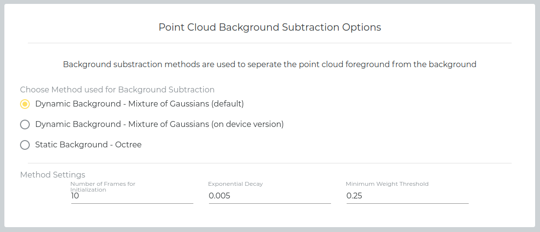
Mixture of Gaussians
Mixture of Gaussians is the default background subtraction. Its benefit is that it can adjust to changing environments. If a new object is placed into the scene and it is remaining there for a certain amount of time it will get merged into the background and will not get recognized anymore/disappears.
Number of Frames for Initialization |
Number of frames used to build the initial background |
Exponential Decay |
Specifies how fast objects switch between foreground and background |
Minimum Weight Threshold |
Controls how much noise the background/foreground is expected to have |
Mixture of Gaussians (on Device)
This option enables the LiDAR to process the background on the device and only send the foreground to Percept. Since this will only send the foreground to Percept, the network traffic is reduced. The degree of data reduction highly depends on how many foreground objects are in the scene.
Number of Frames for Initialization |
Number of frames used to build the initial background |
Exponential Decay |
Specifies how fast objects switch between foreground and background |
| If network traffic is of concern, use this option to reduce network traffic. |
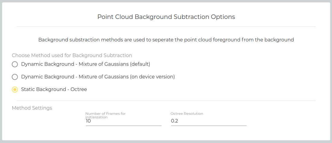
Octree
The Octree option is for static scenes, where no change in the background is expected. It will generate the background when the project is started. The first frames are collected to calculate the background.
Number of Frames for Initialization |
Number of frames used to build the background |
Octree Resolution |
The Octree grid resolution in meters |
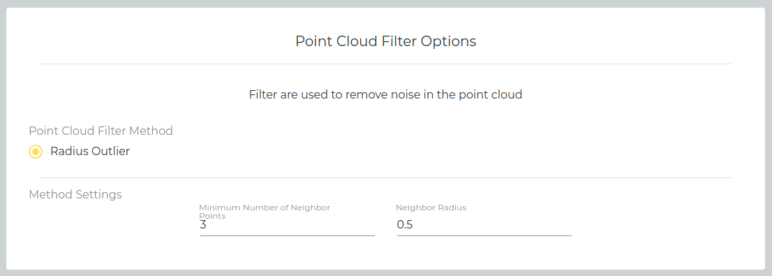
Point Cloud Filter Options
The point cloud filter can remove noise in the scene and therefore improve object detection. The radius outlier filter will eliminate all points that do not have a certain amount of neighbor points in a given radius around that point.
Minimum Number of Neighbor Points |
The minimum number of points in a given radius around that point to be an inlier (valid point) |
Neighbor Radius |
The radius to search for the neighbor points |
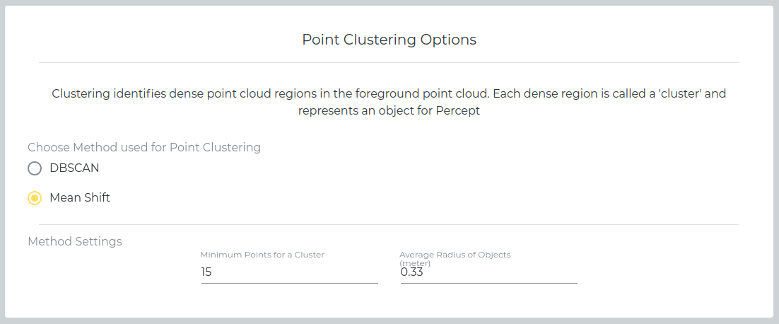
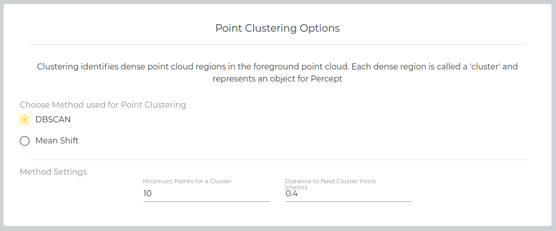
Clustering Options
Clustering identifies dense point cloud regions in the foreground point cloud. Each dense region is called a 'cluster' and Percept considers it as an object. Percept provides several clustering methods.
Mean Shift
For people counting applications we recommend mean shift, since it is very good at separating close circular/spherical objects. But it also requires more processing power in comparison to DBScan.
Minimum Points for a Cluster |
The minimum amount of points to form a cluster |
Average Radius of Objects |
Specifies the average radius of an object in meters |
DBScan
DBScan is less processing intensive compared to Mean Shift and works well for objects with arbitrary shape and size. DBScan performs well on mixed environments with pedestrians, cars and cyclists.
Minimum Points for a Cluster |
The minimum amount of points to form a cluster |
Distance to Next Cluster Point |
Controls how far points are allowed to be separated to belong to the same object-cluster in meters |
-
Set the distance value to the average distance between the LiDAR measurements of the same object. Thereby, the object should be located at the largest distance it still needs to get detected.
-
Set the
minimum pointsto the average amount of points measured within theaverage point distanceidentified in step (1).
If two different objects are detected as one, while they are close to the sensor, increase (2) until objects get separated again. The trade-off is that objects are getting detected only in shorter distances with this configuration.
Tracking Options
The Tracking parameters are set to work with slow objects, like walking people. You can adjust the parameters to your needs. The following parameters are available.
Initial Position Uncertainty |
The expected position error of the first detection of an object |
Initial Velocity Uncertainty |
The expected velocity deviation from zero of newly detected object |
Linear Acceleration Noise |
The expected error with respect to the assumption of having zero acceleration |
Observation Noise |
The expected error of the observed center of an object to the real unobservable center |
-
Increase these values if objects enter the scene with a higher velocity
-
Start by increasing the
initial velocity uncertainty
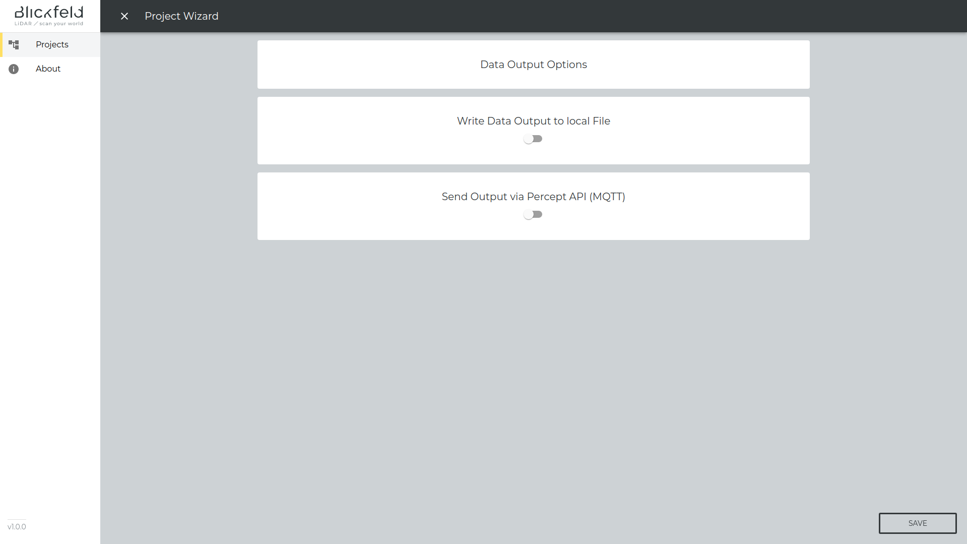
Step 6 - Define Output Options
While you can view the result of the data processed by Percept on the web user interface of Percept, there are also several options to output the data.
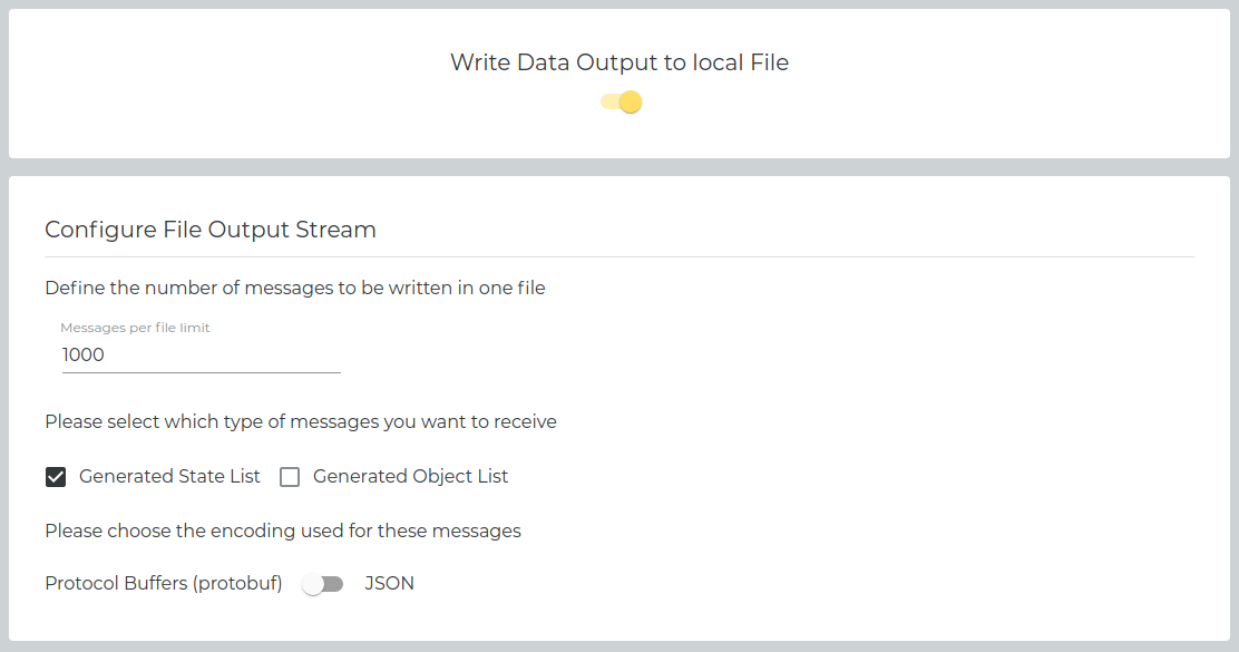
Write to File
Percept can save the detected objects and/or the generated states (e.g. an alarm) to files. The following options are available.
Messages per file limit |
Choose how many messages to write into one file |
Generated State List |
Write the state list to file |
Generated Object List |
Write the object list to file |
Encoding |
Switch between Protobuf or Json as encoding option |
The files can be found in your Percept directory under /data/projects/project_uuid/file_stream/.
|
You can get the ProjectUUID of your project while hovering with your mouse over the icon next to the project name in the overview, see image below. 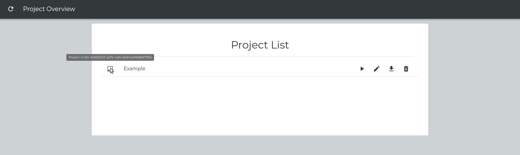
Figure 47. How to find the ProjectUUID of your Project
As an alternative you can also export the zone list, there you will also find the project name and UUID inside the downloaded file. |
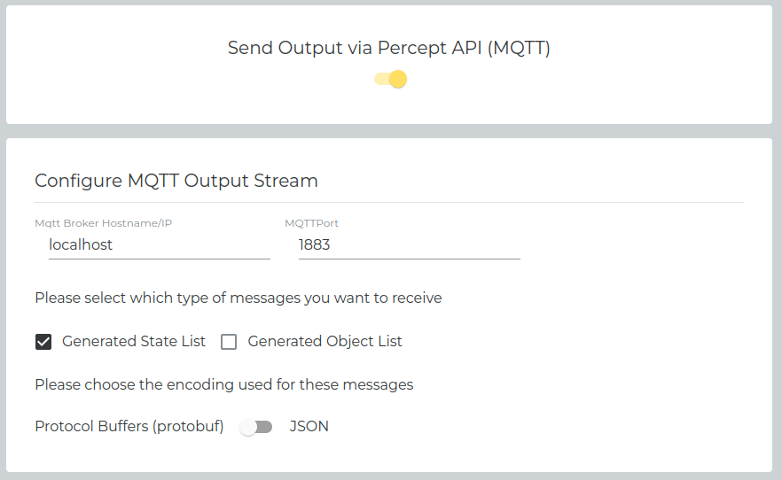
MQTT Publisher
Percept can send the detected objects and/or the generated states to an MQTT Broker. The following options are available.
MQTT Broker Hostname/IP |
The hostname or IP of your MQTT Broker |
MQTT Port |
The MQTT Broker port |
Generated State List |
Write the state list to file |
Generated Object List |
Write the object list to file |
Encoding |
Switch between Protobuf or Json as encoding option |
| Make sure that the MQTT Broker is running before starting your project. Percept itself will not start an MQTT Broker. |
You will receive the MQTT messages on the following Topics, e.g. for Json encoding:
-
blickfeld/project_uuid/json/Statelist
-
blickfeld/project_uuid/json/Objectlist
|
You can get the ProjectUUID of your project while hovering with your mouse over the icon next to the project name in the overview, see image below.
Figure 49. How to find the ProjectUUID of your Project
As an alternative you can also export the zone list, there you will also find the project name and UUID inside the downloaded file. |
| You can enter localhost as hostname if the MQTT Broker is running on the same PC as Percept. |
Step 7 - Manage existing Projects
If you are finished creating your project, you will be redirected to the project overview. There you will find your newly created project, which you can
-
Start
-
Edit
-
Download the zone and point cloud configurations
-
Delete
Start your Project
If you click on the play button, the project will be started. It will generate the selected output and run until you stop it.
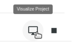
After starting your project a button will appear to visualize and stop the project. If you click on the visualization button, you will get redirected to a visualization page, where you can see the generated Point Cloud of the LiDAR device/s used and the status messages generated by the configured zones, see Visualize your Project for details.
Edit your Project
Percept allows you to change the following parts of your configured Project:
-
Edit Project Name (to rename your project)
-
Edit Zone Configuration (to add/delete/change/rename the zones in your project)
-
Edit Advanced Settings (to change algorithm parameters for your project)
-
Edit Data Output Options (to enable/disable/change the data output options of your project)
The interface is the same as in the setup phase described above.
Download the Zone and Point Cloud Configuration
You can select what configuration to download. Either the zone configuration, point cloud transformation, or both. The output format can be Protobuf or JSON. See Output Encoding Description for a description of the output encoding.
The zone configuration might be helpful:
-
If you want to get the zone position into your application
The point cloud transformation might be helpful:
-
If you want to export the transformation of the point cloud to use in third-party analysis tools.
-
If you want to use the same transformation for another project/application
Delete your Project
Removes your created project.
| If you delete your Project it will get removed and cannot be restored! |
Visualize your Project
The project visualization will use the 3D viewer to show you the point cloud and the detection zones of a running project. This allows you to obtain a live overview about what is happening in the scene and if the setup/configuration is working as intended.
| The visualization does not need to be active to run a project |
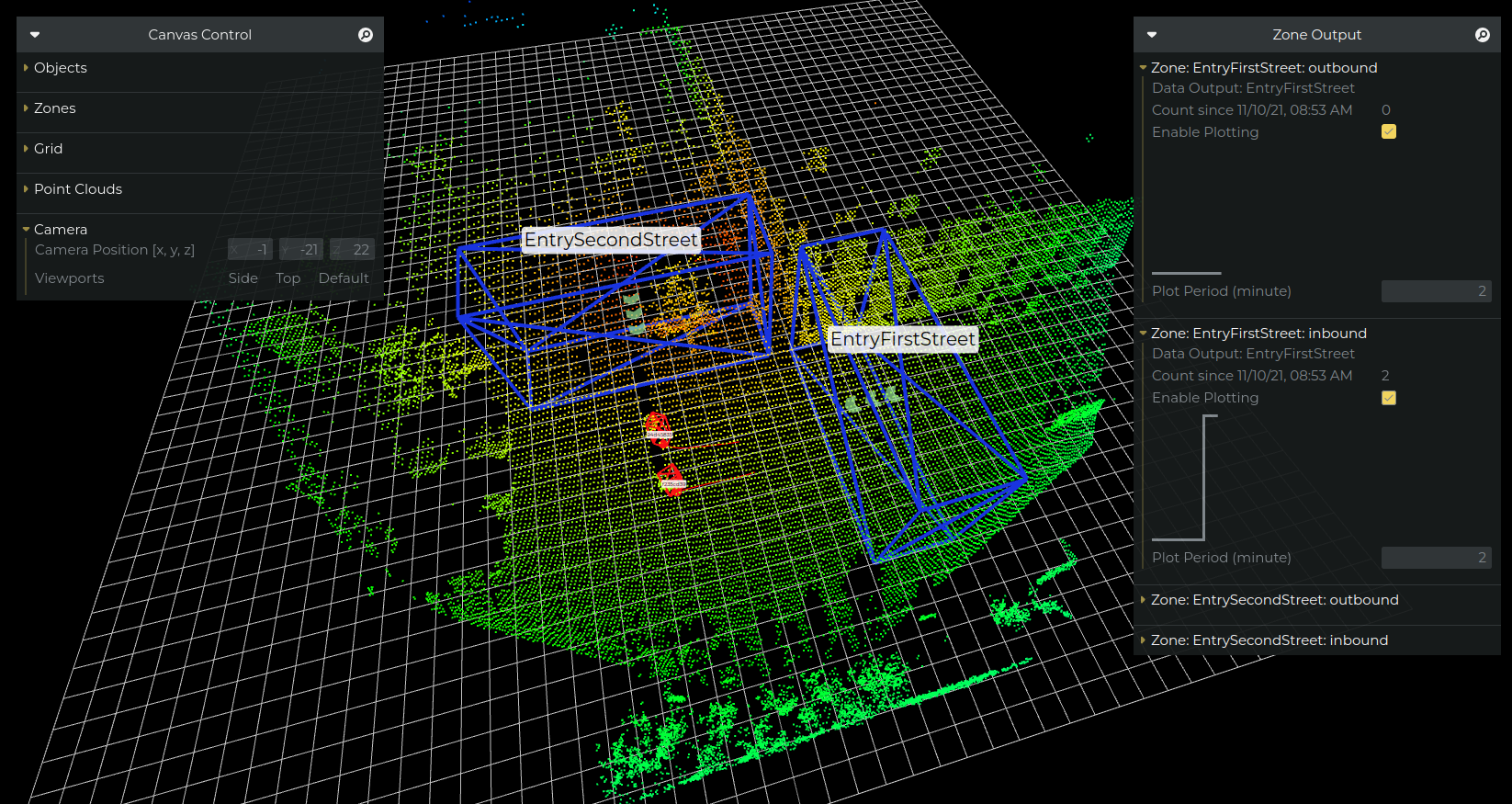
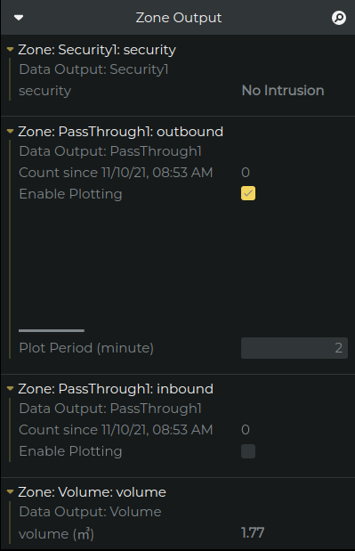
Visualize Zone Output
In the right corner of the project visualization, there is a status display which shows the zone output. Depending on the zone type the following information will be displayed on it.
-
Counter state: it has a number that shows either the accumulated or instant count.
-
Accumulated count: it accumulates the count of the previous states and plots the total value.
-
"Enable Plotting": enable/disable plotting
-
"Plot": plots the accumulated count
-
"Plot Period(minute)": indicating the time slot that the plot will be visualized for, e.g. 2 minutes means the plot will visualize the result of accumulated count for the time frame of 2 minutes.
-
-
Instant count: it visualizes the instant value of the counter and plots the value.
-
For plotting, it has the same parameter as accumulated count
-
-
-
Event state: it will be generated by the event zones and it triggers an event such as:
-
security: "Intrusion"/"No Intrusion"
-
occupancy: "Full"/"Empty"
-
-
Measuring state: it will be generated by the measurement zones and contain the measured value such as:
-
Volume measurement: measured volume in an area
-
Dynamic Services
It is possible to set parameters or request a certain action from the running projects.
-
Tare volume: gives the option to tare the volume during runtime. See Volume Measurement Zone for more information.